Autocallables explained: Structure, risk, and modeling choices that move the price

In the first half of 2026, the US structured notes market booked $119.8 billion in notional across 34,897 products, according to SRP data, and autocallables accounted for 51% of US volume in February alone. 

Why does a product this widely traded remain one of the hardest in equity derivatives to price and hedge well? Dr. Ping Sun, SVP and Head of Quantitative Research at Numerix, took up that question in a recent Numerix webinar, Twenty Years of Autocallables Meet Agentic AI.

The core difficulty is path dependency. Because an autocallable's value rests on the probability of hitting a set of barriers on future observation dates, its price is highly sensitive to the volatility dynamics a model assumes.

Inside an autocallable

Sun described autocallables as equity-linked structured notes that pay above-market yields in exchange for giving up downside protection. In option terms, the note can be viewed roughly as a bond, combined with a short down-and-in put, a short up-and-out autocall option, and coupon features. BNP Paribas issued the first US autocallable in August 2003, and Sun noted that the structure now represents roughly 40% of the global equity structured products market by issuance volume, with particular popularity in Europe and South Korea.

Three barriers define the payoff. The autocall trigger usually sits near 100% of the initial level and often steps down over time. The coupon barrier typically sits between 70% and 90%. The knock-in, or protection, barrier generally falls between 50% and 70% and can be observed at maturity (European) or continuously (American). Coupons may be fixed, conditional (Phoenix), or memory coupons that pay out missed payments once the underlying is above the coupon barrier again.

The risks each side is really holding

From the investor's seat, Sun broke the exposure down into four parts. Investors are short the autocall, short the downside put, short dividends, and, in worst-of baskets, long correlation.

• Short the autocall: A higher forward raises the chance of early redemption, which means losing future coupons. The effect of volatility depends on where the trigger sits relative to the forward: with the trigger near the forward, higher volatility slightly lowers the chance of being called on a given date, while with the trigger well above the forward it raises it.
• Short the down-and-in put: A lower forward or higher volatility increases the probability of knock-in, exposing the investor to losses at maturity.
• Short dividends: Higher dividends lower the forward, which raises the probability of knock-in and also lowers the probability of early call. The knock-in effect usually dominates, so the note loses value, but the net sign depends on how close the underlying is to each barrier.
• Long correlation: In worst-of baskets, higher correlation means less dispersion among the underlyings and a lower chance that any one name breaches the barrier.

The last two exposures are less obvious, and both have produced real losses, though on different sides. Sun pointed to the European dividend cancellations of 2020, when dealers who were long dividends through their autocallable books faced significant losses as expected dividends disappeared. He also cited Korean equity-linked securities tied to the Hang Seng China Enterprises Index (HSCEI), which diverged sharply from co-underlyings such as the EuroStoxx 50 and S&P 500 in 2015 to 2016 and, more severely, in 2021 to 2024, and which hurt long-correlation investors.

Issuers sit on the other side of each of these exposures. They are long the downside put, long dividends, short correlation, and they must hedge Greeks that grow increasingly unstable as the underlying approaches a barrier, particularly near an observation date or maturity.

Why tomorrow's smile sets today's price

The central modeling insight was that an autocallable's value depends on the volatility smile the market will show at future observation dates, conditional on the note not having been called. Getting today's vanilla smile right is necessary but not sufficient.

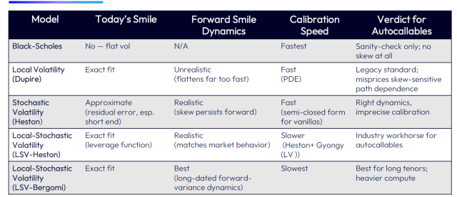
Black-Scholes, with flat volatility, serves only as a sanity check. Local volatility (Dupire) fits today's smile exactly and calibrates quickly, but its implied forward smile flattens far faster than smiles behave in practice. Heston stochastic volatility produces realistic forward skew but, with roughly five parameters to fit the whole surface, cannot fit every maturity’s smile precisely. 

Local-stochastic volatility (LSV) in Heston form combines an exact fit to today's surface with realistic dynamics. Sun described it as the industry workhorse for autocallables, at the cost of slower calibration. For tenors of around five years or longer, he recommended considering LSV with Bergomi-style dynamics, which better captures long-dated forward-variance behavior but carries a heavier computational cost.

The model menu: Strengths & weaknesses

What the stress tests reveal

Dividend and correlation risk are two of the exposures least visible in a term sheet, but they can have a significant impact on how an autocallable behaves. To show how these risks play out in practice, Sun priced a simplified two-year worst-of autocallable on the S&P 500, Nasdaq 100, and Russell 2000 in Numerix CrossAsset, using real market data. The note pays a 2.5% quarterly coupon above a 75% barrier, autocalls at 100%, and carries a European knock-in put struck at 75%. The structure strips out the return of notional so the effect of each shock is easier to read. What remains is the coupon stream less the knock-in put loss, so its present value is close to zero and can be either sign.

Shocking dividend yields by -10 to +10 percentage points produced the expected pattern. At large negative shocks, an early call becomes nearly certain and the models converge near zero. At large positive shocks, the downside put dominates and the models separate, with Heston producing the lowest value, local volatility the highest, and LSV in between. A correlation sweep from -30% to 100% showed value rising with correlation, since a perfectly correlated basket behaves like the single worst underlying, with the widest model divergence at high correlation. Running 50,000 quasi-Monte Carlo paths, the LSV valuation took about 12.6 seconds on CPU and about 2.8 seconds on a laptop-grade GPU.

The term sheet is only the starting point

The Numerix payoff script in Sun's example replaced the hard step function at each barrier with a narrow call spread, which smooths the discontinuity for pricing and reflects how many traders prefer to hedge. Desks also commonly shift a barrier slightly away from its contractual level to tame the delta and gamma singularities that appear near a barrier close to maturity. Neither adjustment appears in a term sheet, and both have to be captured deliberately.

With issuance at record levels and new wrappers such as autocallable ETFs reaching a broader investor base, the distance between a fast price and a defensible one carries more weight. Model choice, dividend and correlation exposure, and barrier treatment all move the number in ways a term sheet will not reveal on its own.

See autocallable pricing in practice

Watch the full replay of Twenty Years of Autocallables Meet Agentic AI to see Dr. Ping Sun's complete walkthrough of autocallable structures, model choice, and risk analysis, along with a live demonstration of agentic AI building and pricing an autocallable trade with Numerix CrossAsset.